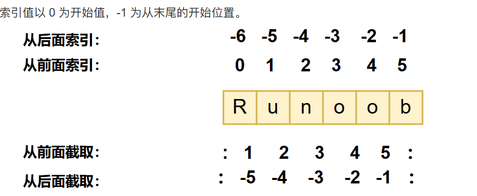
基础语法 基础
整除// 幂**
''和""的使用完全相同,"""可以指定一个多行的字符串,不支持单字符类型,单个字符也视为字符串
\转义符,使用r可以让反斜杠不发生转义
默认输出会自动换行,不需要换行在变量的末尾加上end="",print( x, end=" " )
Nubmber包含int、float、complex(复数)其中int包含bool(True、False)
删除del,del var1[,var2[,var3[....,varN]]]
切片时包含前索引不包含后索引
导入:
将整个模块(somemodle)导入,格式为: import somemodule
从某个模块中导入某个函数,格式为:from somemodule import somefunction
从某个模块中导入多个函数,格式为: from somemodule import firstfunc, secondfunc, thirdfunc
将某个模块中的全部函数导入,格式为:from somemodule import *
运算优先级:
**
幂
~ + -
取反 一元加减号
* / % //
乘,除,取模和取整除
+ -
加法减法
>> <<
右移,左移运算符
&
位 运算符符
^ |
位运算符
<= < > >=
比较运算符
== !=
等于运算符
= %= /= //= -= += *= **=
赋值运算符
数据结构 list列表 列表内的元素可以修改
1
2
3
4
5
6
7
8
9
10
11
12
13
14
15
16
17
18
list = []list .append('Google' )list .append('Runoob' )del list [1 ]list [0 ]='www' len ([1 ,2 ,3 ])print ([1 ,2 ,3 ]+[4 ,5 ,6 ])1 ,2 ,3 ]*2 3 in [1 ,2 ,3 ] print (list ) list .extend([1 ,2 ,3 ])list .count('Google' ) list .insert(2 ,'he' )list .index('he' )list .remove('he' )list .pop(1 )list .sort()list .reverse()
tuple元组 定义时使用小括号且元组内的元素不可修改,访问元组内的元素与列表相同,删除只能删除整个元组
如果你想创建只有一个元素的元组,需要注意在元素后面添加一个逗号 ,以区分它是一个元组而不是一个普通的值,这是因为在没有逗号的情况下,Python会将括号解释为数学运算中的括号,而不是元组的表示。
1
2
3
4
5
tup1 = ('Google' , 'Runoob' , 1997 , 2000 )type (tup1)1 , 2 , 3 , 4 , 5 )list = list (tup3)
dictionary字典(map) 表示映射关系的键(key)值(value)对,key必须唯一,键不可变,因此可以使用数字,字符串,元组而不能使用列表
1
2
3
4
5
6
7
8
9
tinydict = {'name' : 'runoob' , 'likes' : 123 , 'url' : 'www.runoob.com' }len (tinydict)type (tinydict)'name' ]'age' ]=7 str (tinydict)del tinydict['name' ]del tinydict
set集合 是一种无需、可变的数据类型,用于存储唯一的元素,创建格式parame = {value01,value02,...}或者set(value)
1
2
3
4
5
6
7
8
9
10
11
12
13
14
15
set1 = {1 , 2 , 3 , 4 } set ([3 , 4 , 5 , 6 ]) 3 in set1 5 ) tuple =(6 , 7 )tuple ) 6 , 7 ]) print (set1)7 ) 8 )
函数 动态参数 使用关键词 *args 接收任意数量的位置参数,存储为元组(tuple)。
1
2
3
4
5
6
7
8
def func (*args ):print (args) 22 )22 ,33 )22 ,33 ,99 )
使用关键词 **kwargs 接收任意数量的关键字参数,存储为字典(dict)
1
2
3
4
5
6
7
def func (**kwargs ):print (kwargs) "猪悟能" )"猪悟能" ,age=18 )"猪悟能" ,age=18 ,email="xx@live.com" )
tips:
1 2 3 4 5 6 7 8 9 10 11 12 13 14 15 16 def func1 (*args, **kwargs ):print (args, **kwargs)def func2 (a1, a2, a3, *args, **kwargs ):print (a1, a2, a3, args, **kwargs)def func3 (a1, a2, a3, a4=10 , *args, a5=20 , **kwargs ):print (a1, a2, a3, a4, a5, args, kwargs)11 , 22 , 33 , 44 , 55 , 66 , 77 , a5=10 , a10=123 )
return 当在函数中未写返回值 或 return 或 return None ,执行函数获取的返回值都是None
return后面的值如果有逗号,则默认会将返回值转换成元组再返回。
1
2
3
4
5
def func ():return 1 ,2 ,3 print (value)
传参 在 Python 中,函数参数的传递方式本质上是 传递对象的引用(内存地址)
不可变对象 (int, str, tuple 等):
函数内修改参数 不会影响外部变量
因为修改时会创建新对象
可变对象 (list, dict, set 等):
函数内 原地修改 (如 append/update)会影响外部变量
函数内 重新赋值 (如 = [])不会影响外部变量
本质 :参数传递的是内存地址的副本,但操作方式决定了是否共享内存
函数式编程 map函数 1 2 3 4 5 6 >>> def f (x ):... return x * x>>> r = map (f, [1 , 2 , 3 , 4 , 5 , 6 , 7 , 8 , 9 ])>>> list (r)1 , 4 , 9 , 16 , 25 , 36 , 49 , 64 , 81 ]
reduce函数 1 2 3 4 5 6 >>> from functools import reduce>>> def add (x, y ):... return x + y>>> reduce(add, [1 , 3 , 5 , 7 , 9 ])25
过滤序列filter 1 2 3 4 5 def is_odd (n ):return n % 2 == 1 list (filter (is_odd, [1 , 2 , 4 , 5 , 6 , 9 , 10 , 15 ]))
列表生成式 1 2 >>> list (range (1 , 11 ))1 , 2 , 3 , 4 , 5 , 6 , 7 , 8 , 9 , 10 ]
海象运算符 py==3.8后引入的新的赋值表达式运算符,可以在表达式中进行赋值操作,符号为:=
1 2 3 4 5 6 7 8 9 10 11 12 13 14 15 16 17 18 19 input ("Enter a line: " )while line != "quit" :print (f"You entered: {line} " )input ("Enter a line: " )while (line := input ("Enter a line: " )) != "quit" :print (f"You entered: {line} " )for x in range (10 ):if y > 10 :for x in range (10 ) if (y := x * x) > 10 ]
面向对象 1 2 3 4 5 6 7 8 9 10 11 12 13 14 15 16 17 18 19 20 21 22 23 24 25 26 27 28 29 30 31 32 33 class Employee :'所有员工的基类' 0 "" 0 def __init__ (self, name, salary ): self .name = nameself .salary = salary1 def displayCount (self ): print ("Total Employee %d" % Employee.empCount)def displayEmployee (self ):print ("Name : " , self .name, ", Salary: " , self .salary)def updateEmployee (self, name, salary ):self .name = nameself .salary = salarydef __del__ (self ): self .__class__.__name__print (class_name, "销毁" )self .displayEmployee()"John" , 1000 )"Mike" , 1500 )"Alex" , 2000 )
继承 1 2 3 4 5 6 7 8 9 10 11 12 13 14 15 16 17 18 19 20 21 22 23 24 25 26 27 28 29 30 31 32 33 34 35 36 37 38 39 40 41 42 43 44 45 46 47 48 49 class people :'' 0 0 def __init__ (self,n,a,w ):self .name = nself .age = aself .__weight = wdef speak (self ):print ("%s 说: 我 %d 岁。" %(self .name,self .age))class student (people ):'' def __init__ (self,n,a,w,g ):self ,n,a,w)self .grade = gdef speak (self ):print ("%s 说: 我 %d 岁了,我在读 %d 年级" %(self .name,self .age,self .grade))class speaker ():'' '' def __init__ (self,n,t ):self .name = nself .topic = tdef speak (self ):print ("我叫 %s,我是一个演说家,我演讲的主题是 %s" %(self .name,self .topic))class sample (speaker,student):'' def __init__ (self,n,a,w,g,t ):self ,n,a,w,g)self ,n,t)def speak (self ):print ("%s 说: 我 %d 岁了,我在读 %d 年级,我演讲的主题是 %s" %(self .name,self .age,self .grade,self .topic))"Tim" ,25 ,80 ,4 ,"Python" )super (sample,test).speak() print (sample.__mro__)
类 特殊方法/魔法方法 定义了类要如何对待运算符的python内置函数的方法,往往前后有两个下划线,叫作dunder method->double underscore
import 导入文件时的查找是根据执行目录sys.path来的
假设我们A导入B,在B导入C,BC在同目录下,运行A,当前目录是A所在的目录,虽然BC是同级,但无法直接导入
导入时的*可用__all__来定义
1 2 3 4 from packageA import *'X' ,'moduleA' ]
相对导入
**单个点 (.)**:表示当前包。
**两个点 (..)**:表示当前包的父包。
**三个点 (...)**:表示当前包的父包的父包,以此类推。
例如,假设有以下目录结构:
1 2 3 4 5 6 my_package/ __init__ .py test1.py sub_ package/ __init__.py test2.py
在 test2.py 中,你可以使用相对导入来导入 test1.py 中的函数:
1 from ..test1 import devide
为了使相对导入正常工作,请确保:
你的代码在包的上下文中运行。
使用 -m 选项从包的根目录运行 Python 解释器。
__init__.py
包的初始化
管理包的接口
1 2 3 4 from packageA import *'X' ,'moduleA' ]
管理包的信息
1 2 __version__='1.0.0' 'cwdpsky'
NumPy 安装
pip install numpy或conda install numpy
n维数组对象ndarray 创建ndarray对象,只需调用 NumPy 的 array 函数即可:
1 numpy.array(object , dtype = None , copy = True , order = None , subok = False , ndmin = 0 )
参数说明:
名称
描述
object
数组或嵌套的数列
dtype
数组元素的数据类型,可选
copy
对象是否需要复制,可选
order
创建数组的样式,C为行方向,F为列方向,A为任意方向(默认)
subok
默认返回一个与基类类型一致的数组
ndmin
指定生成数组的最小维度
实例 接下来可以通过以下实例帮助我们更好的理解。
实例 1
1 2 3 import numpy as np 1 ,2 ,3 ]) print (a)
输出结果如下:
实例 2
1 2 3 4 import numpy as np 1 , 2 ], [3 , 4 ]]) print (a)
输出结果如下:
实例 3
1 2 3 4 import numpy as np 1 , 2 , 3 , 4 , 5 ], ndmin = 2 ) print (a)
输出如下(注意这里有两层中括号,意味着这是一个二维数组):
实例 4
1 2 3 4 import numpy as np 1 , 2 , 3 ], dtype = complex ) print (a)
输出结果如下:
数组属性 NumPy 数组的维数称为秩(rank),秩就是轴的数量,即数组的维度,一维数组的秩为 1,二维数组的秩为 2,以此类推。
在 NumPy中,每一个线性的数组称为是一个轴(axis),也就是维度(dimensions)。比如说,二维数组相当于是两个一维数组,其中第一个一维数组中每个元素又是一个一维数组。所以一维数组就是 NumPy 中的轴(axis),第一个轴相当于是底层数组,第二个轴是底层数组里的数组。而轴的数量——秩,就是数组的维数。
很多时候可以声明 axis。axis=0,表示沿着第 0 轴进行操作,即对每一列 每一行
NumPy 的数组中比较重要 ndarray 对象属性有:
属性
说明
ndarray.ndim数组的秩(rank),即数组的维度数量或轴的数量。
ndarray.shape数组的维度,表示数组在每个轴上的大小。对于二维数组(矩阵),表示其行数和列数。
ndarray.size数组中元素的总个数,等于 ndarray.shape 中各个轴上大小的乘积。
ndarray.dtype数组中元素的数据类型。
ndarray.itemsize数组中每个元素的大小,以字节为单位。
ndarray.flags包含有关内存布局的信息,如是否为 C 或 Fortran 连续存储,是否为只读等。
ndarray.real数组中每个元素的实部(如果元素类型为复数)。
ndarray.imag数组中每个元素的虚部(如果元素类型为复数)。
ndarray.data实际存储数组元素的缓冲区,一般通过索引访问元素,不直接使用该属性。
ndarray.ndim ndarray.ndim 用于获取数组的维度数量(即数组的轴数)。
1 2 3 4 5 6 7 import numpy as np 24 ) print (a.ndim) 2 ,4 ,3 ) print (b.ndim)
输出结果为:
ndarray.shape ndarray.shape 表示数组的维度,返回一个元组,这个元组的长度就是维度的数目,即 ndim 属性(秩)。比如,一个二维数组,其维度表示”行数”和”列数”。
ndarray.shape 也可以用于调整数组大小。
1 2 3 4 5 6 7 import numpy as np 1 ,2 ,3 ],[4 ,5 ,6 ]]) print (a.shape)3 ,2 ) print (a)
输出结果为:
1 2 3 4 (2 , 3 )[[1 2] [3 4] [5 6]]
NumPy 也提供了 reshape 函数来调整数组大小
1 2 3 4 5 import numpy as np 1 ,2 ,3 ],[4 ,5 ,6 ]]) 3 ,2 ) print (b)
输出结果为:
NumPy创建数组 numpy.empty 1 numpy.empty(shape, dtype = float , order = 'C' )
在使用 numpy.empty 创建数组时,数组中的元素是未初始化的内存值,既不是 0,也不保证是任何特定值,而是取决于当时内存的残留数据(可能是随机值、垃圾值或之前程序残留的数据)。
参数说明:
参数
描述
shape
数组形状
dtype
数据类型,可选
order
有”C”和”F”两个选项,分别代表,行优先和列优先,在计算机内存中的存储元素的顺序。
1 2 3 import numpy as np 3 ,2 ], dtype = int ) print (x)
输出结果为:
numpy.zeros 创建指定大小的数组,数组元素以 0 来填充:
1 numpy.zeros(shape, dtype = float , order = 'C' )
参数说明:
参数
描述
shape
数组形状
dtype
数据类型,可选
order
‘C’ 用于 C 的行数组,或者 ‘F’ 用于 FORTRAN 的列数组
1 2 3 4 5 6 7 8 9 10 11 12 13 import numpy as np5 ) print (x)5 ), dtype = int ) print (y)2 ,2 ), dtype = [('x' , 'int' ), ('y' , 'float' )]) print (z)
输出结果为:
1 2 3 4 [0. 0 . 0 . 0 . 0 .]0 0 0 0 0 ]0 , 0 .) (0 , 0 .) (0 , 0 .)]0 , 0 .) (0 , 0 .) (0 , 0 .)]]
numpy.ones 创建指定形状的数组,数组元素以 1 来填充:
1 numpy.ones(shape, dtype = None, order = 'C ')
参数说明:
参数
描述
shape
数组形状
dtype
数据类型,可选
order
‘C’ 用于 C 的行数组,或者 ‘F’ 用于 FORTRAN 的列数组
1 2 3 4 5 6 7 8 9 import numpy as np5 ) print (x)2 ,2 ], dtype = int )print (x)
输出结果为:
1 2 3 [1. 1. 1. 1. 1. ][[1 1] [1 1]]
numpy.zeros_like numpy.zeros_like 用于创建一个与给定数组具有相同形状的数组,数组元素以 0 来填充。
numpy.zeros 和 numpy.zeros_like 都是用于创建一个指定形状的数组,其中所有元素都是 0。
它们之间的区别在于:numpy.zeros 可以直接指定要创建的数组的形状,而 numpy.zeros_like 则是创建一个与给定数组具有相同形状的数组。
1 numpy.zeros_like(a, dtype=None , order='K' , subok=True , shape=None )
参数说明:
参数
描述
a
给定要创建相同形状的数组
dtype
创建的数组的数据类型
order
数组在内存中的存储顺序,可选值为 ‘C’(按行优先)或 ‘F’(按列优先),默认为 ‘K’(保留输入数组的存储顺序)
subok
是否允许返回子类,如果为 True,则返回一个子类对象,否则返回一个与 a 数组具有相同数据类型和存储顺序的数组
shape
创建的数组的形状,如果不指定,则默认为 a 数组的形状。
创建一个与 arr 形状相同的,所有元素都为 0 的数组:
1 2 3 4 5 6 7 8 9 import numpy as np1 , 2 , 3 ], [4 , 5 , 6 ], [7 , 8 , 9 ]])print (zeros_arr)
输出结果为:
1 2 3 [[0 0 0] [0 0 0] [0 0 0]]
numpy.ones_like numpy.ones_like 用于创建一个与给定数组具有相同形状的数组,数组元素以 1 来填充。
numpy.ones 和 numpy.ones_like 都是用于创建一个指定形状的数组,其中所有元素都是 1。
它们之间的区别在于:numpy.ones 可以直接指定要创建的数组的形状,而 numpy.ones_like 则是创建一个与给定数组具有相同形状的数组。
1 numpy.ones_like(a, dtype =None, order ='K' , subok =True , shape =None)
参数说明:
参数
描述
a
给定要创建相同形状的数组
dtype
创建的数组的数据类型
order
数组在内存中的存储顺序,可选值为 ‘C’(按行优先)或 ‘F’(按列优先),默认为 ‘K’(保留输入数组的存储顺序)
subok
是否允许返回子类,如果为 True,则返回一个子类对象,否则返回一个与 a 数组具有相同数据类型和存储顺序的数组
shape
创建的数组的形状,如果不指定,则默认为 a 数组的形状。
创建一个与 arr 形状相同的,所有元素都为 1 的数组:
1 2 3 4 5 6 7 8 9 import numpy as np1 , 2 , 3 ], [4 , 5 , 6 ], [7 , 8 , 9 ]])print (ones_arr)
输出结果为:
1 2 3 [[1 1 1] [1 1 1] [1 1 1]]
pandas pandas是基于NumPy的数据分析库,提供了高性能、易用的数据结构和数据分析工具。
安装:pip install pandas 或 conda install pandas
数据结构 Series(一维数据) Series是一种类似于一维数组的对象,由数据和索引组成。
1 2 3 4 5 6 7 8 9 10 11 12 13 14 15 import pandas as pdimport numpy as np1 , 3 , 5 , np.nan, 6 , 8 ])print (s1)1 , 2 , 3 , 4 ], index=['a' , 'b' , 'c' , 'd' ])print (s2)'a' : 1 , 'b' : 2 , 'c' : 3 }print (s3)
DataFrame(二维数据) DataFrame是二维的表格型数据结构,有行索引和列索引。
1 2 3 4 5 6 7 8 9 10 11 12 13 'Name' : ['Alice' , 'Bob' , 'Charlie' ],'Age' : [25 , 30 , 35 ],'City' : ['New York' , 'Paris' , 'London' ]print (df)'20240101' , periods=6 )6 , 4 ), index=dates, columns=list ('ABCD' ))print (df2)
数据操作 数据查看 1 2 3 4 5 6 7 8 9 10 11 12 13 14 15 16 17 18 19 20 21 3 )
数据选择 1 2 3 4 5 6 7 8 9 10 11 12 13 14 15 'Name' ] 'Name' , 'Age' ]] 0 ] 0 ] 0 :2 ] 0 :2 , 'Name' :'Age' ] 'Age' ] > 25 ]'City' ].isin(['New York' , 'Paris' ])]
数据修改 1 2 3 4 5 6 7 8 9 10 11 'Salary' ] = [50000 , 60000 , 70000 ]0 , 'Age' ] = 26 'Salary' , axis=1 , inplace=True )0 , axis=0 , inplace=True )
数据处理 处理缺失值 1 2 3 4 5 6 7 8 9 10 11 12 1 ) 0 ) 'ffill' )
数据分组和聚合 1 2 3 4 5 6 7 8 9 10 'City' )sum ()'City' ).agg({'Age' : 'mean' , 'Salary' : 'sum' })
数据合并 1 2 3 4 5 6 7 1 ) 'key' ) 'key' , how='left' )
文件读写 1 2 3 4 5 6 7 8 9 'data.csv' )'data.xlsx' )'data.json' )'output.csv' , index=False )'output.xlsx' , index=False )'output.json' )
Scikit-Learn Scikit-Learn是Python中最流行的机器学习库,提供了各种监督和无监督学习算法。
安装:pip install scikit-learn 或 conda install scikit-learn
基本工作流程 1 2 3 4 5 6 7 8 9 10 11 12 13 14 15 16 17 18 19 20 21 22 23 24 25 26 27 28 29 30 31 32 from sklearn.model_selection import train_test_splitfrom sklearn.preprocessing import StandardScalerfrom sklearn.linear_model import LinearRegressionfrom sklearn.metrics import mean_squared_error, r2_scoreimport pandas as pdimport numpy as npfrom sklearn.datasets import load_boston0.2 , random_state=42 )print (f'MSE: {mse} , R²: {r2} ' )
常见算法 线性回归 1 2 3 4 5 6 7 8 9 10 11 12 13 from sklearn.linear_model import LinearRegression, Ridge, Lasso1.0 )1.0 )
逻辑回归 1 2 3 4 5 6 7 8 9 10 11 12 13 14 15 16 17 from sklearn.linear_model import LogisticRegressionfrom sklearn.datasets import load_iris0.2 , random_state=42 )from sklearn.metrics import accuracy_score, classification_report, confusion_matrixprint (f'Accuracy: {accuracy_score(y_test, y_pred)} ' )print (classification_report(y_test, y_pred))
决策树 1 2 3 4 5 6 7 8 9 from sklearn.tree import DecisionTreeClassifier, DecisionTreeRegressor5 , random_state=42 )5 , random_state=42 )
随机森林 1 2 3 4 5 6 7 8 9 10 11 12 from sklearn.ensemble import RandomForestClassifier, RandomForestRegressor100 , random_state=42 )100 , random_state=42 )
支持向量机 1 2 3 4 5 6 7 8 9 from sklearn.svm import SVC, SVR'rbf' , C=1.0 )'rbf' , C=1.0 )
K-均值聚类 1 2 3 4 5 6 7 8 9 from sklearn.cluster import KMeansimport matplotlib.pyplot as plt3 , random_state=42 )
数据预处理 特征缩放 1 2 3 4 5 6 7 8 9 10 11 12 13 from sklearn.preprocessing import StandardScaler, MinMaxScaler, RobustScaler
特征编码 1 2 3 4 5 6 7 8 9 from sklearn.preprocessing import LabelEncoder, OneHotEncoderfrom sklearn.preprocessing import get_dummies'category_column' ])
模型评估 交叉验证 1 2 3 4 5 6 7 8 9 10 from sklearn.model_selection import cross_val_score, KFold5 )print (f'CV scores: {scores} ' )print (f'Mean CV score: {scores.mean()} (+/- {scores.std() * 2 } )' )5 , shuffle=True , random_state=42 )
网格搜索 1 2 3 4 5 6 7 8 9 10 11 12 13 14 15 16 from sklearn.model_selection import GridSearchCV'n_estimators' : [50 , 100 , 200 ],'max_depth' : [3 , 5 , 7 ],'min_samples_split' : [2 , 5 , 10 ]5 )print (f'Best parameters: {grid_search.best_params_} ' )print (f'Best score: {grid_search.best_score_} ' )
学习曲线 1 2 3 4 5 6 7 8 9 10 11 12 13 14 15 from sklearn.model_selection import learning_curve5 , train_sizes=np.linspace(0.1 , 1.0 , 10 )10 , 6 ))1 ), label='Training score' )1 ), label='Validation score' )'Training Size' )'Score' )
管道(Pipeline) 1 2 3 4 5 6 7 8 9 10 11 12 13 14 15 16 17 18 19 20 21 22 from sklearn.pipeline import Pipeline'scaler' , StandardScaler()),'classifier' , RandomForestClassifier())'classifier__n_estimators' : [50 , 100 ],'classifier__max_depth' : [3 , 5 ]5 )
机器学习 分类
肯定类别
否定类别
阳性判断
真阳性记录数TP
假阳性记录数FP
阴性判断
假阴性记录数FN
真阴性记录数TN
精确率:precision=$\frac{TP}{TP+FP}$,表示预测为正的样本中有多少是真正的正的样本
召回率:recall=$\frac{TP}{TP+FN}$,表示预测为正且正确的样本占预测为正的比例
支持向量机(SVM)